 Aaron Beaudoin
Astrophysics
Research
Before UX, I studied astronomy and astrophysics at the University of Illinois. These are two projects from that time: one on exploding stars, one on software I wrote to test ALMA's radio receivers.
Searching for Imprints of Circumstellar Material in the Ultraviolet Spectra of Type Ia Supernovae
Type Ia supernovae (SNe Ia) are thermonuclear explosions that have high and relatively standard peak luminosities. It is accepted that SNe Ia originate in white dwarf (WD) binary systems, however, the companion star is still unclear. Two possible progenitor models are the single- (SD) and double-degenerate (DD) scenarios, where the companion in the DD scenario is another WD, while the companion in the SD scenario is a more normal star such as a red giant.
Here, we test these models by searching for indications of circumstellar material (CSM) in Hubble Space Telescope UV spectra of 8 SNe Ia. Imprinted on these UV spectra are narrow absorption lines from ISM and/or CSM. If these features vary in strength over time, the material is likely CSM, ionizing and recombining after the SN explosion. Such material is most easily explained in a SD progenitor system. Using a total of 46 spectra from 8 SNe Ia, we do not detect any variability in Mg I, Mg II, and Fe II lines, placing new, strong constraints on the progenitor systems of these SNe Ia.
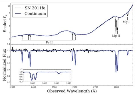
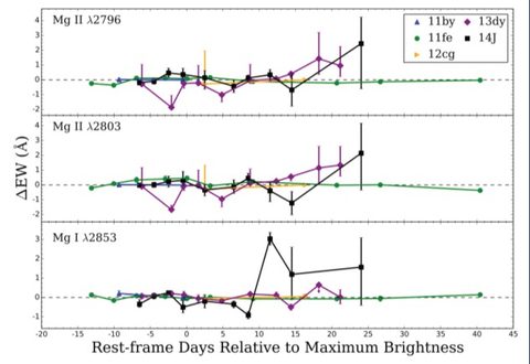
We detect the Mg II λ2800 doublet and Mg I λ2853 in all spectra, although SNe 1992A, 2011ek, and 2011iv only show absorption from the Milky Way. We also detect Fe II in some observations from each SN. Measuring the EW of each feature at each epoch, we look for any variability. In our best measurements to date, we do not detect any significant change in any of the absorption features, consistent with studies of optical features for SN 2011fe (Patat et al., 2013) and SN 2014J (Welty et al., 2014; Goobar et al., 2014, Foley et al., 2014). We therefore do not detect a large amount of CSM along our line of sight.
References
- Patat et al., 2013, A&A, 549, 62.
- Welty et al., 2014, ApJ, 792, 2.
- Goobar et al., 2014, ApJL, 784 12.
- Foley et al., 2014, MNRAS, 433, 2887.
Modular Analysis Software for the ALMA Front End Test and Measurement System
Introduction
The Atacama Large Millimeter/ Submillimeter Array (ALMA) is a radio interferometer that is located in the Atacama Desert in Chile (altitude ~16,400 ft.). It consists of 66 antennae, creating a synthesized aperture with a diameter of up to 16 km. There are 59 12-m antennae and seven 7-m antennae, each of which has a parabolic dish (cannot deviate from a perfect parabola by more than 20 microns), sub-reflector, and receiver.
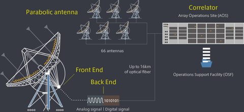
The Front End: Each front end is a cryogenically cooled system that has 10 receiver bands that allow a frequency coverage from 31.3 GHz to 962 GHz. Each band, except bands 1 & 2, is cooled to 4 K and consists of an orthomode transducer (OMT) and either a pair of SIS mixers (bands 3-7) or a single SIS mixer (bands 8-10) that are fed by a 90° hybrid RF coupler and LO couplers. This structure can be seen in Figure 2. This system essentially takes a sky signal and 1) mixes it with a reference frequency generated by a local oscillator (LO), 2) lowers the signal to an intermediate frequency (IF), 3) splits it between its polarizations (using the OMT), then splits it again into an upper and lower sideband (using the SIS mixers), and 4) sends these signals to the back end.
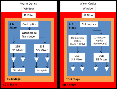
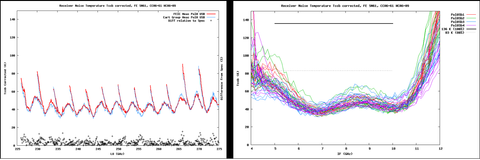
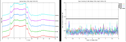
The Test System: The test system compares system outputs to pre-determined specifications for minimal noise in the observations made by the receivers. This system tests noise temperature (noise added to the output from the receiver) and the IF output spectrum (checks for spikes in power over the IF window and the maximum power variation a specified IF range), along with other attributes in the Warm Cartridge Assembly (WCA).
New Modular Library: This library is written in PHP and is used to accept, analyze, and display test data from the Front Ends. This upgrade features a more structured interface that allows flexible database retrieval, universal data structures that allows for simple data manipulation, and an adaptable plotting algorithm.